The neighbourhood of two adjacent vertices in a Conway 99-graph

In the previous post, we saw that if a is a vertex of a Conway 99-graph G, then up to labelling the only possibility for the neighbourhood of v is the following:

An arbitrary vertex 0 has 14 neighbours, which can be arranged in pairs a,a+1 such that the only edges are: 0,a; 0,a+1; a,a+1 for odd a.

In this post, we describe the results of a search for all possible subgraphs consisting of two adjacent vertices a,b and all of their neighbours in G.

The route

Suppose there exists a Conway-99 graph G, that is, an SRG(99,14,1,2). Let a and b be vertices of G such that a and b are neighbours. Then:

  • a has 14 neighbours, one of which is b
  • b has 14 neighbours, one of which is a
  • By λ = 1, precisely one of these neighbours is a mutual neighbour of both a and b

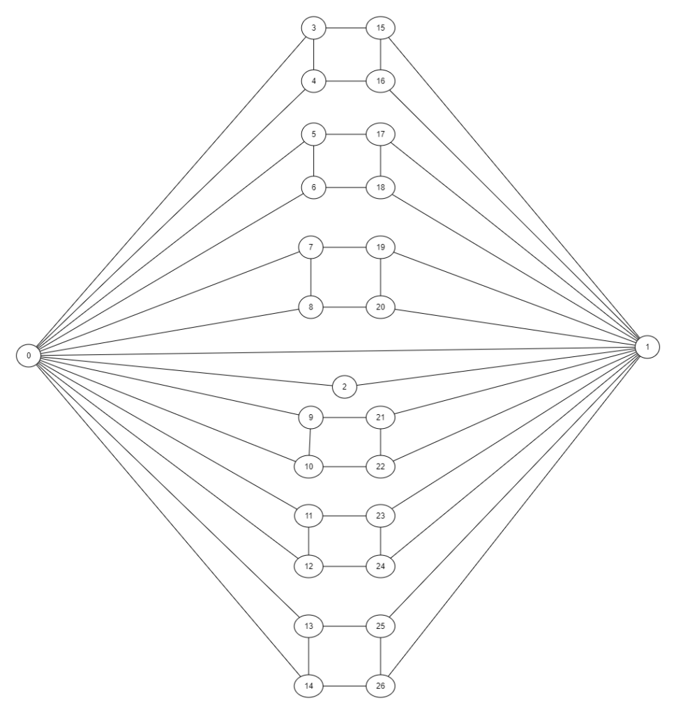
Thus the graph G’ on a,b and their neighbours consists of 27 vertices (a, b, their mutual neighbour, 12 neighbours of a but not b, and 12 neighbours of b but not a). For convenience, we fix a numbering:

  • a is vertex 0
  • b is vertex 1
  • Their mutual neighbour is vertex 2
  • The remaining neighbours of vertex a are vertices 3 through 14
  • The remaining neighbours of vertex b are vertices 15 through 26

Moreover, we introduce these vertices sequentially using the ‘fanblade’ structures centred at vertices 0 and 1:

  • For i,j in 1…14 we have i,j adjacent iff j = i + 1 and i is odd (as in the diagram above)
  • For i,j in 15…26 we have i,j adjacent iff j = i + 1 and i is odd
  • (The seventh blade for vertex 1 consists of vertices 0 and 2)

Finally, we note that each of the vertices i = 15…26 is not adjacent to vertex 0, thus (by μ = 2) there must be two mutual neighbours of 0,i in G. But as all neighbours of 0 are in G’, namely vertices 1…14, we know that each vertex i = 15…26 is adjacent to precisely 2 of the vertices 1…14.

  • By assumption, vertex 1 is adjacent to vertex i
  • Hence vertex 2 is not adjacent to vertex i (else 0 and i and are mutual neighbours of adjacent vertices 1 and 2, which violates λ = 1)
  • So for each i = 15…26 there is a unique j in 3…14 such that i and j are neighbours.
  • For the first such i=15, all choices of j give equivalent graphs on vertices 0…15. Wlog, we set j=3.
  • Our task then essentially reduces to determining j for each i=16…26, whilst satisfying all our other conditions.

The code

I have produced an assortment of python functions for working efficiently with strongly regular graphs, defaulting to the Conway 99-graph but (hopefully) valid for generic parameters; a public github repository is here. Included is a notebook working through this search; you can view it here if you just want the results without having to run the code yourself.

The rest of this section sketches out some of the challenges in working with srgs, particularly with regard to growing valid supergraphs from a given starting set.

‘Growing’ subgraphs

Adding vertices

As discussed in the previous post, we could in principle work our way from any subgraph G’ to G by considering all possible ways to add a vertex v’ to G’, and discarding those which can be identified as breaching a known subgraph property.

In practice we can terminate even sooner. Consider our starting subgraph N(0) on vertices 0…15. We know that vertex 0 is ‘saturated’ in that all of its neighbours are already present. So any proposed addition of vertex 16 which sets the edge (0,16) is doomed to failure; we should recognise this once rather than try all of the 32,768 possible combinations of (1,16), (2,16), (3,16) …, (15,16).

Matrix representation

Thus far we’ve described everything purely in graph-theoretic terms. However, graphs can be awkward to work with as a data structure; under the hood, we will instead use two dimensional arrays for the corresponding adjacency matrix of a graph.

Usually, this is a matrix of 0s and 1s where the (i,j)th entry is 1 if and only if vertices i and j are adjacent. (Thus when we say the adjacency matrix, we actually mean an adjacency matrix – for an unlabelled graph each choice of vertex numbering will give different – but equivalent – representatives. For this search, however, we have already prescribed a particular labelling.)

However, in the code we’ll extend this to a template form which also allows (i,j) to take the value 2, to indicate an unspecified edge and thus a collection of graphs sharing some common edges and non-edges.

A round of growing

Thus, given a set S of potential n-vertex subgraphs of G, we can grow to the set of potential (n+1)-vertex subgraphs as follows.

For each g in S:

  • Form an (n+1) by (n+1) all-twos matrix a’.
  • Set values a[0,0] through a[n-1,n-1] using the adjacency structure on vertices 0…n-1 given by g.
  • Set the diagonal entry a'[n,n] = 0 (as the new vertex n cannot be a neighbour of itself).
  • For any required edge between vertex n and some vertex i of g, set a'[i,n] and a'[n,i] = 1.
  • For any required non-edge between vertex n and some vertex i of g, set a'[i,n] and a'[n,i] = 0.
  • Add a’ to the template list.

Then, whilst the template list is not empty:

  • Remove any a’ from the template list.
  • Identify the lowest indices i,j such that a'[i,j]=2.
  • Construct new arrays a0 and a1, by first copying a’ but then setting a0[i,j]=a0[j,i]=0 and a1[i,j]=a1[j,i]=1
  • If a0 is a purely 0,1 array then check whether the corresponding graph violates any of the subgraph properties described in the previous post. If not, add it to the solution list.
  • Otherwise, a0 is a template. However, we may already be able to rule it out, if the edges and non-edges specified thus far already specify an invalid feature (for example a vertex of degree 15, or a second mutual neighbour of vertices known to be adjacent). If no such features exist, add a0 to the template list.
  • Perform the previous two steps for a1 in the same way (if an adjacency matrix, add to solution list if valid; if a template, add to template list if not already invalid).

This process necessarily terminates. If the solution list is empty, we have proven that G cannot have any g from S as a subgraph. Conversely, if the solution list S’ is non-empty, we can treat this as a new S and repeat the procedure.

If we knew that at least one of the g in S was a necessary subgraph of G, then if S’ is empty we know that G does not exist. If S’ is nonempty, we now know that at least one of the g’ in S’ is a necessary subgraph of G. Unfortunately, there may be a huge number of these!

Reducing subgraphs

Fortunately, many of them will turn out to be equivalent, as we can take alternative routes to the same (abstract) graph. For example, we argued at the start that attaching vertex 15 to any of j = 3 through 14 was equivalent, so we might as well specify that j it be vertex 3. If we hadn’t done that, we would have obtained 12 valid solutions, one for each choice of j. Having done so, our specification of vertex 16 as the mutual neighbour of vertices 1 and 15 yields 11 solutions, but these only fall into two equivalence classes.

Thus we need to be able to reduce the solution list modulo isomorphism. For the mathematical part I rely upon Nauty, via the orthogonal array package; this documentation (implicitly) describes how to compare a single pair of matrices for equivalence by comparing if they have the same normal form.

It’s easy enough to wrap this comparison up in a function on a pair of arrays. Then the solution list can be reduced by building up a representative list, adding each entry of the solution list only if it is inequivalent to all representatives added so far.

However, this soon turns out to be prohibitively expensive to compute (even with early abort when a match is found), due to the need to put both the representative and the candidate in normal form each time. It is better, therefore, to keep the normal forms along with the representatives, then normalise each candidate once and test for equality to any of the representative normal forms. Since we’re now testing equality, we can go faster by handling this as a dictionary lookup rather than sequentially working through a list… except numpy arrays are mutable and thus can’t be used as keys. Thus I took the questionable choice of converting the normalised array to a full tuple of its entries to get something hashable, likely losing all sorts of representational efficiency: a classic time/memory trade-off that has made the reduction pass negligble compared to the proceeding growing step, but will eventually cause problems!

Validity Testing

One final area where refinement proved necessary was in checking adjacency matrices or templates for invalid features. Given the size of the graphs I was able to work with, the eigenvalue constraints never came into play, so all that is implemented in the code is checks for vertices with excessive degree, adjacent vertices with more than one mutual neighbour, or non-adjacent vertices with more than two mutual neighbours.

As with equivalence testing, it’s pretty easy to write functions that compute the numbers of common neighbours, but when comparing in bulk there is simply too much repeated or otherwise unnecessary work: when you add a vertex to a valid graph, there are only a few places where it can become invalid; and as soon as you find one invalid vertex pair there’s no need to continue testing others. Thus in the code you can find _with_subgraph_mutuals versions of various functions, which again trade off some memory to avoid recomputing known (or more easily derived) values.

The Results

With these various improvements, it takes only a few seconds to recover the possible 27-vertex graphs on 0,1 and their neighbours.

There turn out to be only eleven possibilities. The first of these proceeds in the obvious way, matching 16 to 4, 17 to 5 and so on for this pleasing (after some artistic re-arrangement in yEd!) graph:

The others are more complicated; the notebook describes the differences to this baseline. We can also see that there are no edges in common to all 11; that is, our initial choices did not propagate further and we require further assumptions to force a particular subset of the solutions.

Searching further

Unfortunately, things get much worse from here. The github repo contains two ‘full search’ notebooks. The first proceeds as with our route, trying to introduce neighbours of vertex 2; this will climb to nearly 3 million 33-vertex graphs which it is unable to reduce. The second hands control over edge requirements to a ‘greedy’ version of the growing algorithm, which identifies the vertex closest to being saturated and attempts to add neighbours of that (in the hopes of reaching impossible features sooner). Tiebreaking on label, this therefore favours vertex 3 over vertex 2 but grinds to a halt sooner, at 31 vertices.

I also attempted a sampling rather than exhaustive search: this throws away all but a tiny portion of the results each round in the hope of finding a route through by chance. Unsurprisingly, this has not yielded anything, although the vertex counts attained can be decent.

Finally, it’s natural to ask for the graph consisting of two non-neighbours and their respective neighbours. This sounds like a very minor tweak on what we’ve done here: we add vertex 15 a first non-neighbour of 0, then proceed to saturate it instead of vertex 1. But this too falls victim to acombinatorial explosion of possibilities – whilst it has not yet outright crashed, I expect days of cputime to complete it.

So, for now, I offer this up for others to consider. Perhaps these 11 graphs contain enough information for a mathematical argument rather than trying to push on computationally; or perhaps some of the code I’ve written will be helpful. But if not, it was enjoyable playing around with some ‘proper’ maths for a while, and to overcome the series of programming puzzles presented by each of the search, reduction and validity checking bottlenecks.
Constraints on Conway’s 99-graph (and its subgraphs)

In the previous post, we introduced strongly regular graphs, with a particular interest in whether an srg(99,14,1,2) could exist. In this post, we’ll look at some properties such a graph G – or various subgraphs G’ – would have to satisfy.

(throughout, we’ll use G to refer to any Conway 99-graph, and use ‘subgraph’ to describe graphs obtained by vertex deletions only – sometimes called proper or induced subgraphs – rather than the more general concept which allows edge deletions too.)

The degree of every vertex is necessarily 14

First, then, we should make good on the promise to prove that the degree parameter k is 14, since Conway’s formulation of the problem only specifies the number of vertices and the mutual neighbour parameters λ=1, μ=2.

For this, we’ll use a double counting argument – expressing the same number in two different ways, and equating those expressions. For this, pick any vertex of G and call it vertex 0. Then as G is assumed to be regular, 0 has k neighbours, wlog vertices 1…k. Let A be the set of vertices 1…k, and B be the set of vertices k+1…98 (i.e. all the vertices apart from 0 and its neighbours). The quantity we will count is the number of edges between vertices in A and vertices in B.

  • First, consider any vertex i in A. As a neighbour of vertex 0, they must have precisely one neighbour in common; since all the neighbours of 0 are in A, so there must be an edge from i to precisely one other i’ in A. Apart from the edge linking i to 0, all other edges starting at A must be to vertices in B. For vertex i to have degree k, there must therefore be k-2 edges from vertex i to B. Our choice of vertex i was arbitrary from A, which contains k vertices; so in total there are k(k-2) edges from A to B.
  • Conversely, consider any vertex j in B. j is not a neighbour of vertex 0, so they must have 2 mutual neighbours; necessarily those are vertices of A (else they don’t neighbour 0 either). Thus each of our 98-k vertices k+1…98 contributes 2 edges from B to A, for a total of 2(99-k-1) = 196 – 2k.
  • Since the edges from A to B are precisely the edges from B to A, we have equality: k(k-2) = 196 – 2k. So k^2 = 196, which for positive k forces k=14 as claimed.

The neighbourhood of each vertex is a seven-bladed fan

Implicit in the above was a description of the neighbourhood of any vertex v of G – that is, the subgraph N(v) consisting of that vertex and all of its neighbours. Let 0 be an arbitrary vertex and pick any neighbouring vertex, calling that vertex 1. Then as 0 and 1 are neighbours, they have precisely one mutual neighbour; wlog vertex 2. This gives us a ‘fanblade’ consisting of vertices 0,1,2: neither vertex 1 nor 2 can have any other neighbours in N(0). We can repeat this process to introduce the vertices in pairs 3-4, 5-6, 7-8, 9-10, 11-12 and 13-14. Thus N(0) is a seven-bladed fan:

An arbitrary vertex 0 has 14 neighbours, which can be arranged in pairs a,a+1 such that the only edges are: 0,a; 0,a+1; a,a+1 for odd a.

Up to labelling, N(v) for any v in G is of this form.

Eigenvalue constraints

We will not prove these results here, but any strongly regular graph has precisely 3 eigenvalues whose values and multiplicities are determined by v,k,λ,μ. For our parameters, the eigenvalues of G are therefore:

  • 14, with multiplicity 1
  • 3, with multiplicity 54
  • -4, with multiplicity 44

The interlacing theorem therefore gives strong requirements on the eigenvalues of sufficiently large subgraphs G’ of G. Recall that if A is an n-vertex graph with eigenvalues a_1…a_n and B is obtained from A by deleting a vertex, then the eigenvalues b_1…b_(n-1) of B interlace with the eigenvalues of A:

a_1 ≤ b_1 ≤ a_2 ≤ … ≤ a_(n-1) ≤ b_(n-1) ≤ a_n

For G we have a_1 = a_2 = …. = a_44 = -4, a_45 = a_46 = … = a_98 = 3, a_99 = 14. So if G’ is a 98 vertex subgraph of G, almost all of its eigenvalues are known too: b_1 through b_43 must be -4, and b_45 through b_97 must be 3. The only freedom is in b_44, which can take values in [-4,3]; and b_98, which can take values in [3,14].

Iterating this process, we arrive at the following corollaries:

Let G’ be any subgraph of G. Then:

  • e≥ -4 for any eigenvalue e of G’
  • e≤ 14 for any eigenvalue e of G’
  • If e>3 is an eigenvalue of G’, then e has multiplicity 1
  • There cannot be two eigenvalues e,e’ of G’ such that e’ > e > 3.

Let G’ be a subgraph of G with n vertices. Then:

  • If n ≥ 56, then n-55 of the eigenvalues of G’ must take the value -4
  • If n ≥ 46, then n-45 of the eigenvalues of G’ must take the value 3

Subgraph compatibility with strong regularity

Let a,b be vertices of a subgraph G of G’. If a and b are neighbours in G’, then they are neighbours in G, so there must exist precisely one c in G adjacent to both a and b. If a and b are not neighbours in G’, then they are not neighbours in G either (by our notion of subgraph); so there must exist precisely two vertices d,e in G adjacent to both a and b. However, these vertices c,d,e need not feature in G’ – their absence is not reason to discard G’ as a potential subgraph of G.

Conversely, if a proposed G’ has too many mutual neighbours, then this can never be ‘fixed’ by adding more vertices, so we can rule out such a subgraph. Thus we have:

Let G’ be a subgraph of G. Then:

  • If a and b are adjacent vertices in G’, then they have at most one mutual neighbour in G’
  • If a and b are non-adjacent vertices of G’, then they have at most two mutual neighbours in G’

However, these mutual neighbours must eventually be introduced, and so we can additionally rule out candidate subgraphs where we have missed this opportunity:

Let G’ be a subgraph of G containing a vertex a and all of its neighbours in G, a_1…a_14. Then:

  • Each a_i must neighbour precisely one other a_j
  • For any b in G’ not amongst the a_i (or a itself), b must be a neighbour of precisely two of the a_i

Finally, we have the trivial observation that the regularity condition also restricts G’:

Let a be a vertex of a subgraph G’ of G. Then a has degree at most 14.

~

In the next post we’ll attempt to ‘grow’ our way towards G from a subgraph – we won’t get far enough to make use of our eigenvalue constraints, but we are able to enumerate the possibilities for the subgraph consisting of two adjacent vertices and their combined neighbourhoods. Before that, though, I wanted to note in passing some other properties of the Conway graph that I found during my research, although I don’t know how I would test for them…

Group-theoretic restrictions

  • From “On the (99,14,1,2) strongly regular graph” (pp. 342-355 of this collection), if G exists, it does not have an automorphism of order 11, which implies that the automorphism group cannot be transitive.
  • Example 3.2 of this paper gives the critical group of G.

Conway’s 99-graph (and related problems)

I have been on furlough for the last six weeks, which has given me the time to engage properly with a research-grade problem I have been thinking about on-and-off for a number of years! Spoiler alert: this series of posts is not building up to the grand reveal of a solution, but instead is intended to summarise what I’ve learnt and perhaps help ease the way of the next person to give it a try.

Earlier this year, COVID-19 claimed one of mathematics’ greats, John Horton Conway. The Guardian’s obituary does a far better job than I could of illustrating his remarkable range of major contributions across the subject, whilst this MathOverflow post collects together a wonderful assortment of lesser results (including, wonderfully, his ‘discovery’ of the filing cabinet).

But a mathematician lives on in their questions as well as their solutions, and in 2014 Conway had curated five particular problems, an answer to any of which would be rewarded with a thousand dollar prize. I first learnt of this list in 2017, when a counterexample was found by James Davis to the fifth entry, the ‘climb to a prime’ conjecture. Davis is rather unfairly described as an ‘amateur’ in what little coverage I could find of this achievement; but at least that gave me hope that I wouldn’t be completely wasting my time in checking the rest of the list!

Sure enough, the second problem caught my eye as something which, in principle, could be tackled in a similar way to the questions I considered back in my academic research days. Conway’s statement is as follows:

Is there a graph with 99 vertices in which every edge (i.e. pair of joined vertices) belongs to a unique triangle and every nonedge (pair of unjoined vertices) to a unique quadrilateral?

It seems that there are other ways to (mis?)interpret this statement, but in more formal terms this is asking

Does there exist a strongly regular graph with 99 vertices and parameters λ=1, μ=2?

So, what does that mean, and what hope might we have of finding such objects?

Strongly Regular Graphs

For integers v,k,λ,μ a graph G is described as being an srg(v,k,λ,μ) if it satisfies all of the following:

  • G has v vertices
  • G is regular – the degree (number of neighbours) of every vertex is fixed – and moreover that degree is k
  • if two vertices are neighbours, they have precisely λ mutual neighbours
  • but if they are not neighbours, they instead have precisely μ mutual neighbours

Thus Conway’s problem is asking for an srg(99,k,1,2). As we’ll see in the next post, only carefully chosen combinations of the four parameters have any chance of yielding a solution. In this case setting v=99, λ=1 and μ=2 is already enough to force a single possibility for the degree k; if Conway’s 99-graph exists, it’s an srg(99,14,1,2). However, it need not be unique – there can be non-isomorphic graphs satisfying the same choice of parameters (and so a natural follow-up challenge given one example is a complete enumeration up to isomorphism).

SRGs with λ=1, λ=2

In fact, Conway’s choice of λ=1, μ=2 is already highly restrictive, with only five possibilities.

  • Simplest is the (unique) srg(9,4,1,2):

    srg(9,4,1,2)

    To me, this is the Paley graph of order 9; such graphs capture information about finite fields, with applications to number theory. But in addition, it’s: a conference graph; toroidal; locally linear; and the graph of the triangular duoprism (from 4 dimensional geometry). It also represents the possible moves of a rook on a 3-by-3 chessboard. Quite a lot for 9 vertices and 18 edges!

  • The next smallest possibility is the Conway 99-graph.
  • From there, we jump to an srg(243,22,1,2). Remarkably, this does exist, and can be constructed by tying together ideas from coding theory, group theory and graph theory. The result is the Berlekamp–van Lint–Seidel graph, which I won’t attempt to draw!
  • The other two possibilities remain open problems:

    Does an srg(6273,112,1,2) exist?

    Does an srg(494019,994,1,2) exist?

Small SRGs

Through a variety of smart search techniques (some of which we’ll consider in the next post), it has been possible to test all the potential parameters corresponding to small strongly regular graphs, where small currently means at most 64 vertices; see the collection of Ted Spence. As the Berlekamp–van Lint–Seidel graph shows, there are larger parameter choices for which strongly regular graphs are known to exist. There are also potentially valid parameters for larger graphs whose existence has been ruled out – for instance, there is no srg(96,38,10,18), but that fact does not immediately follow from the parameters.

Andries E. Brouwer maintains a summary of the possibilities and their current status. From there, we note that the following remains open

Does an srg(65,32,15,16) exist?

But a resolution in the negative (or a full description if solutions do exist) would extend the classification to graphs of at most 68 vertices (as we already know of the 66 vertex examples, and that there are no suitable parameters for 67 or 68 vertices).

A hypothetical Moore graph

As these examples show, the difficulty of finding (or proving non-existence of) strongly regular graphs does not correspond neatly to the number of vertices. The smaller the other parameters, the fewer edges that need to be considered and thus the easier it is to identify forbidden subgraph structures. The most extreme case is λ = 0 – which requires the graph to be triangle-free – and μ = 1. A strongly regular graph that satisfies both of these conditions would be a Moore graph; the only barrier to our complete understanding of such graphs is the following question:

Does an srg(3250,57,0,1) exist?

~

The existence of a Conway 99-graph (or of any of the other srgs I’ve called out above) is precisely my kind of problem: the statement is easy to understand; a (positive) solution would be easy to verify; but it’s not easy to get from statement to solution! As we’ve seen, in some cases clever constructions can be used to directly manufacture strongly regular graphs, and instances of existing families of graphs may turn out to have strong regularity as a feature. In the next post we’ll consider instead how we might ‘grow’ a solution through careful consideration of a series of subgraphs. As well as being used in the large scale searches of Spence et al, this is precisely the technique I used for my work on (non)cyclotomic graphs back in the day, so I was keen to revisit it and see how far I could get in a different context.

Euro 2018

I’ll be attending the 29th European Conference on Operational Research – more simply, Euro 2018 – in Valencia this summer. I’m not giving a presentation, but as I’ll be attending on behalf of OVO I’d be particularly keen to talk to anyone with experience of applying OR techniques in the energy industry. At a personal level, I’m also keen to learn more about MILP / constraint satisfaction algorithms at scale.

Visualising air quality data with Voronoi diagrams

This is the extended version of my lightning talk from the second PyData Bristol meetup.

The basic idea for this visualisation – using Voronoi diagrams to map air quality data – is one I’ve been carrying around for several years, but only recently did I have the right combination of data, tools, and project time to make it a reality. My new job at OVO required me to dust off my python skills – for which I prefer a toy project to abstract study – and gave me access to Tableau, which meant I could lean on its mapping capabilities and easy sharing of visualisations. Working for a green energy company also seemed more appropriate for shining a light on poor air quality than my previous roles in aviation! Open Data Bristol provided the raw material – although their site seems to be in flux, with the exact dataset I used no longer available – and here’s what I did with it:

Voronoi diagrams in the wild

So what is a Voronoi diagram? Given a particular point from a set of points – in this case, individual air quality monitors set up around Bristol – the Voronoi cell is all the locations which are closer to that point than any of the others. A Voronoi diagram (or tessellation) is then the collection of all these cells; here, it partitions Bristol so that for any location in the city, you can see at a glance the air quality reading from its nearest monitor. This has a more instant impact than just plotting the points: highlighting that poor air quality likely affects broad areas, not just a particular monitor; and eliminating the need to determine the nearest sensor to a place of interest (especially as zooming to a local level of detail may remove monitors from view entirely).

However, I’m not aware of any dataviz programs that offer Voronoi diagrams ‘out of the box’, and indeed, this is not their main field of application. They arise in an impressive variety of domains across mathematics, CS and the natural sciences – and have even found their way into artistic endeavours – so I’m surprised that they don’t appear in undergraduate curricula. Or, at least, they didn’t feature in mine; so here’s a few contexts in which I’ve since encountered them!

Biology

Long-necked Voronoi diagrams

Instead of thinking of Voronoi cells as being constructed, we can imagine them arising organically. If we have growth occurring at the same rate from multiple seed sites, then collisions will occur precisely at the boundaries of the Voronoi cells corresponding to those sites. Similarly, if pigments or other chemicals are spread from the sites, they will meet and react for the first time along those same boundaries. As a result, Voronoi diagrams can be used to model natural phenomena ranging from the skin patterns of giraffes to the structures of tortoise shells or dragonfly wings (Wikipedia has a neat animation of this).

Physics

200801245
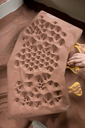
Making Voronoi diagrams with sand

If waiting for biology seems too slow, you can also produce your Voronoi diagrams with physics. In the above example, holes have been drilled into blocks covered with fine sand; once the holes are uncovered from below, some sand will flow through. But grains will drain out from their nearest hole, and are more likely to do so if they’re closer. Thus, once the pile settles, it does so with ridges at the locations furthest from the holes: that is, the boundaries of the Voronoi cells. Similar processes occur in mud cracking, lava cooling or soap bubble formation; these can be thought of as physical optimisation algorithms, where in this case the best solution relates to your nearest or furthest neighbour. (By analogy, we can exploit Voronoi diagrams to answer operational research style problems such as where best to place a new shop or distribution centre.)

Architecture


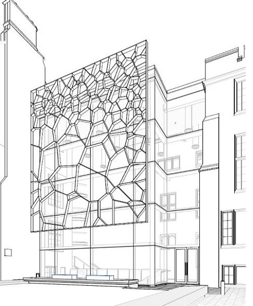
Design for the Fry building, University of Bristol

Voronoi diagrams have become popular in architecture, particularly as screens or roofs, where the irregular cell layout enables a mixture of light and shade patterns (and an alternative, more organic, aesthetic than arises from grid-based designs). A local example will soon be found in pride of place at the University of Bristol’s Fry building, which will be the new home for the School of Mathematics. However, their summary doesn’t specify what it’s a diagram of!

Voronoi diagrams in python

Obtaining Voronoi cells

The mathematics of Voronoi diagrams belongs to discrete and computational geometry, and I highly recommend the book of the same name by Devadoss and O’Rourke – so good, I actually have two copies! This was an area that I dabbled in shortly before I departed academia, and have always wanted to do more with.

Fortunately, python being python, there’s no need to reinvent the wheel. Importing voronoi from scipy.spatial we can easily construct and plot the Voronoi diagram from an array of X,Y pairs describing our points of interest:

The blue points are the original sites, whilst the orange ones are the vertices of the Voronoi cells (or regions as they are referred to here). So at first glance, it might seem that we’re done… but on closer inspection – or rather, further, by expanding our viewing window from the conveniently chosen one – some issues are revealed:

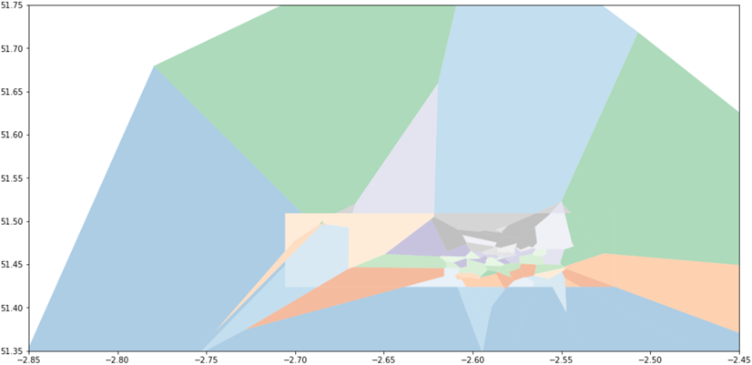
The ‘problem’ is with the outer cells, and mathematically there is no problem at all. Recall that the goal of the Voronoi diagram is to divide up the plane into regions according to their closest site. But this is the idealised mathematical plane: in the simplest case of two starting points, the entire (flat) universe is divided into two infinite halves, separated by the perpendicular bisector of the line through the points. For more complicated collections of points, we get two types of Voronoi cells: the finite ones, with a well defined boundary made up of finite line segments; plus the infinite ones, where borders shared with other infinite cells will be rays that extend indefinitely from a boundary point. In the plots above, these rays are represented by dashed lines rather than the solid boundaries of the finite cells.

The Voronoi methods actually handle this by working with the list of boundary vertices for each region, rather than its ‘shape’. Each orange point we see carries an index, from which we can recover its coordinates in the plane. But there is also a ‘point at infinity’ (with index -1) for which there is no corresponding point; the infinite regions are those which include this point in their vertex list.

Obtaining finite Voronoi cells

For visualisation purposes, we’d like to restrict the cells to fall within some bounding box – in our case, large enough to include all our air quality monitors, but not otherwise stray too far from Bristol. As we’ll soon see, there are python data structures that make this operation straightforward for polygons – but we need to deal with those infinite regions first. The trick is to turn them into large – much larger than our eventual area of interest – but finite polygons first, by projecting those infinite boundary rays out much further before truncating.

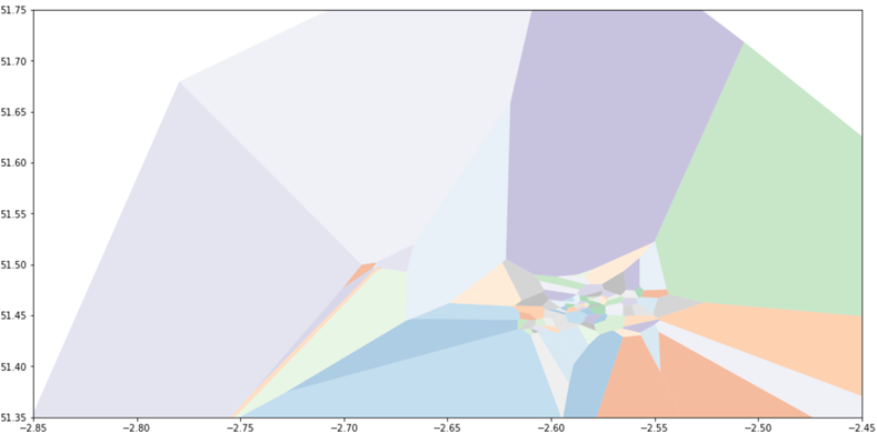
I would like to say I thought through the mathematics for this, but instead I turned to Stackoverflow, suspecting that others had had the same problem. Sure enough, this question – and this solution by user ‘sklavit’ – give us the pieces we need. This plot, on the same axis as before, but now showing individual polygons rather than collections of points and lines – illustrates some of the effect:

Working with shapes in python

Sklavit’s solution actually contains two parts: generating the finite regions as lists of boundary vertices; then using the shapely library to construct Polygons with those boundaries. These can then have geometric operations easily applied to them; in particular, a bounding box polygon can be created and the intersection of this with each Voronoi cell found.

This suffices to demonstrate their solution to the problem. But in practice, working directly with individual polygons can be fiddly – there are issues with shared boundaries, for instance – and for our visualisation purposes we’d need some book-keeping to track which data values correspond to each cell (especially if the original points are no longer contained in any of the bounded polygons).

We can therefore benefit from a more elaborate structure. The geopandas library extends pandas data frames to allow each row to have a geometry (described by a shapely polygon). This allows us to perform set-theoretic operations on collections of shapes en-masse, and get a new collection back. Better still, we can associate our shapes with data and metadata, and this will be carried through to the new shapes as appropriate.

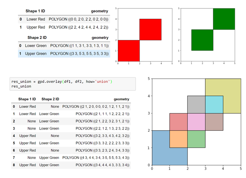
For example, taking the union of overlapping shapely polygons directly only gives us a single larger polygon. With geopandas, we get a collection of polygons which add up to the same result, but track each piece’s relationship with the original polygons. Here’s an illustration of that effect:

For our purposes we can therefore preview the effect of applying a particular bounding box, by considering its union with a geodata frame of the finite cells:

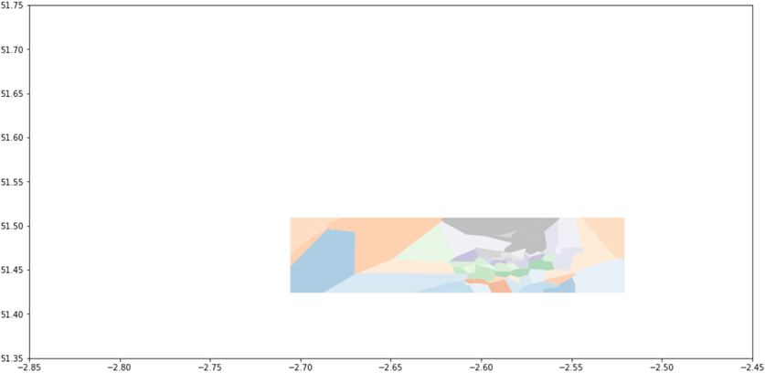
Although, of course, it is the intersection that we actually wish to keep:

where each of the surviving shapes has data columns inherited from the finite cells, which could themselves have been easily associated with monitor data (since shapely allows us to test whether a point is contained in a polygon).

Putting it all together

Working with shapes in tableau

From here we can move to Tableau, provided we can translate to data it understands. This is fairly straightforward, once you’re aware of a few quirks of Tableau’s polygon mark type…

  • A Tableau polygon is defined by a set of boundary points, and we need one data row per point.
  • An index or label is needed to indicate which points belong to which polygon (and should be applied to the detail or colour shelf).
  • An additional path index is needed to indicate the order in which the boundary is constructed from the points (and should be applied to the path shelf).
  • Unlike shapely polygons and, confusingly, tableau’s path mark type, you should not ‘close the loop’ by repeating the initial vertex.

Thus the remaining task in python is to produce these appropriately indexed lists of points. These could then be merged back to the original data in Tableau, but I found it simpler (albeit wasteful of space) to produce a single file, replicating each cell’s data across all its boundary points.

If you wish to be able to plot both the cells and the original sites, then you’ll need to use a dual axis plot in Tableau, and differentiate the two types of geometry (polygon and point) in the data. You’ll also need to hide the boundary points of each cell (or use the shape shelf to render them invisible), since Tableau filters apply to both axes simultaneously. The visualisation above demonstrates this effect if you enable the ‘Show Monitor Locations’ option.

Example notebook

Our recipe is therefore as follows:

  • obtain some data with X,Y coordinates;
  • recover the (potentially infinite) Voronoi regions;
  • reduce these to finite Voronoi cells;
  • truncate these to polygons within a suitable bounding box;
  • convert to a point-by-point format for Tableau.

I’ve implemented each of these steps in a Jupyter notebook, which you can find here. Note that this only produces the output needed for a single Voronoi diagram using the 2016 air quality data, which is (currently) available under the Open Government Licence v3.0. To produce the multi-year visualisation (with a diagram for each year based on the monitors that were active then) I simply iterated this process, and added year as an additional column before concatenating the output and exporting to Tableau; sadly this is no longer available as a single data set!

Limitations

Although I’m happy with this particular visualisation, this code is not suitable for all such uses. This is because the process makes a faulty – but apparently increasingly popular – assumption: that the world is a flat plane! Since we actually live on (roughly) a sphere, this creates a couple of issues when treating longitude and latitude as if they were X,Y coordinates.

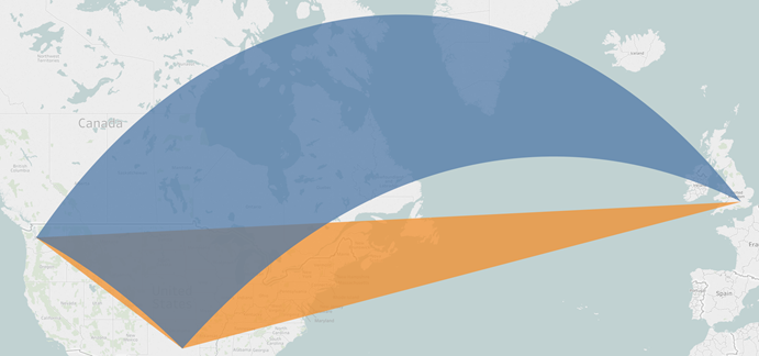
Firstly, we define our Voronoi cells by their boundary vertices, which we then join by a ‘straight’ line. However, the shortest path from one geographic coordinate to another – e.g. an edge of a cell – would be a great circle, which appears as a curve under this projection. Fortunately, this distortion is relatively minor for paths across, say, Bristol. But it is worth keeping in mind at an international scale; this example shows how Tableau (in orange) would render a triangle between three major airports, versus how it would slice a segment out of the globe (in blue):

One solution would be for Tableau’s path rendering to be aware of these issues; alternatively, we could compute these curves in python first and output a much larger number of points to define the boundary of each cell.

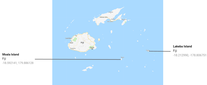
However, treating geographic coordinates as points in a plane will cause much bigger problems elsewhere in the world, regardless of scale:

Had we been attempting to map Fijian rather than Bristolian air quality, we’d have run into difficulties as extremely negative and positive longitudes indicate locations which are close by, not far apart. Although latitude at the poles does not have the same ‘wrap around’ effect, distortion would be pronounced there too.

Fortunately these are known and solved issues, resulting in spherical Voronoi diagrams and some of my favourite visualisations. So if you found all of this straightforward, I’d love to see a python implementation that computes these correctly anywhere on the globe, and can then project them to a map!

Visualisation Of Scottish Demographic Data

My MSc dissertation is available for download here, as a 7.54Mb PDF. Here’s the abstract:

This project explores the use of interactive visualisations to augment the extensive data published by the National Records of Scotland. Good visualisation can illustrate key trends in statistical data, increasing impact and accessibility; great visualisation can go further, and enable us to identify and explore unexpected connections. Data visualisations can therefore support operational research, but we will see that producing them also entails solving problems of an OR flavour.

We survey the existing literature for principles of good design in presenting data visually; much of this is aimed at hand-produced imagery for print, so we examine how it can be best used in the new context of procedurally-generated, interactive visualisations for the web. In the first instance, we consider this for chart types which have proven popular or successful for static visualisations, particularly if already used by NRS.

This leads us to investigate more complicated data sets which can be interpreted as having a graph theoretic structure. We will show how the constrained layout of networks of vertices with an associated size can be posed as an optimisation problem, and develop a visualisation that operates under such constraints. Further, we will consider the use of geographic clustering to represent migration flow, describing and implementing a novel `re-wiring’ algorithm to generate tree structures that produce better visualisations than standard agglomerative approaches.

Finally, we present a portfolio of visualisations created for NRS that follow the design principles identified and make use of the software tools developed during the project.

There is also an online version of the appendix with links to the various visualisations developed, including source code and sample data files. The rest of this post gives at-a-glance versions.

The Cause of Death Explorer

Cause of Death Treemap

Experimental alternative presentation of the above data set; not suitable for Internet Explorer


Fertility
Fertility data (cohort effects)

Baby names
Popular baby names for boys

Also available for girls!

Scottish Life Expectancy
Life Expectancy

The first to be used in NRS reporting, appearing here.

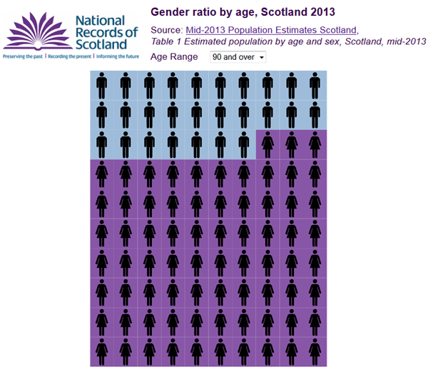
Gender distribution by age

Scottish Migration
Migration chord diagram (experimental)

My Erdős number…

…appears to be four (an infinite improvement). I coauthored a paper with Gary Greaves, whose recent paper Edge-signed graphs with smallest eigenvalue greater than -2 also saw contributions from Jack Koolen and Akhiro Munemasa. They both have an Erdős number of two (each via Chris Godsil, who is an Erdős coauthor), making Gary a three and myself a four.

If I do not publish any more papers, the best I can hope for is three, if Gary later collaborates with a one. But for now my goal should be to obtain a Bacon number…

Recent popular baby names in Scotland

Amelia Pond from Doctor Who

The Scottish Amelia Pond first appeared in Doctor Who in 2010 – is she responsible for the sudden popularity of the name, or did I just want an excuse to use this picture?

Given my previous anthroponomastical adventures I knew I’d want to play around with the popular names datasets during my project. Whilst I should only be thinking about visualisation rather than analysis, spend enough time compiling values from two dozen Excel files and you’ll inevitably start noticing patterns (even when they aren’t really there). So this post will explore some of those too.

The data available is the top 100 names for each of boys and girls born in Scotland, every year 1998-2013 except 2000 (for unknown reasons). For each name that features, the precise count is also given – but for any that fail to make the cut, we don’t have this figure. As well as this censoring effect – for which the precise threshold will vary each year – raw counts should really be considered in the context of varying birth rates too: there may be less children with a particular name simply because there are less children! So for the visualisation project I focused my efforts on the rankings. After various experiments, I settled on simply showing the top 20 each year. Interestingly, this doesn’t require too much data. For example, there are just 25 different boys names that feature in any of the 13 top 10’s; and only another 16 are needed to form the pool for the top 20’s, as many of those are past or future members of the top 10. So, here’s the boys:

and similarly for the girls:

However, I couldn’t resist going back to the raw counts to look at some of these in more detail. For instance, at the top of the charts we seem to have captured “peak Emma“; from highs of around 630 in 2003-04, it not only lost the top spot to Sophie but plummeted out of the top 10 (and nearly the top 20), with just 237 of them a decade later. The shift is even more pronounced when you consider that Sophia cracked the top 20 from 2011, and Sofia is also to be found further down the top 100. For the boys, Lewis has also declined substantially from its chart-topping days, but still holds a top three position despite there being less than half as many in 2013 than 2003.


The Sophie/Sophia/Sofia situation is an example of a rather common phenomenon girls names. Although the truncated rankings will suppress the least popular variants, a sufficiently popular name can carry with it homophones (such as Niamh/Neve1 or Abbie/Abby; Nieve, Abi and Abbi have also featured in top 100’s) or clusters of similar names (Ella/Elle/Ellie, Eva/Eve/Evie) as the next graph shows:

As mentioned, the most popular names usually spend some time as moderately popular ones first, and take a while to disappear entirely. But an interesting example of a name that has very recently sprung into prominence is Amelia. The shorter Amy held a top ten spot for all but two years 2001-2010, and the variant Aimee also made the top 20 for all of 2003-2006 (finding favour slightly later than Amy). But save for the 87th spot in 2005, Amelia was nowhere to be found until 2007; and only made the top thirty for the first time in 2012, somehow leaping straight to ninth place and staying there for 2013 too. Definitely one to watch for 2014!

Finally, I couldn’t resist an egotistical look at the data. However, in a sure sign of my advancing age, neither Graeme nor Graham ever make the top 100 for any of the years available…fortunately in 2013 the complete list was also published, and from this I note seven instances of Graham, three of Graeme (despite that being the more traditionally Scottish spelling), and both a Gray and a Graye too. On the other hand, my surname has the distinction of being reasonably popular as a first name for both boys and girls – the only other unisex example I spotted was Jordan, but that was substantially more common for boys. For Taylor, it’s fairly even – but also falling out of fashion it seems!

1 Yes, those sound the same. Blame gaelic. For bonus marks, can you pronouce 2007’s twentieth most popular name, Eilidh?